
Batch Score - Excel™ Cheat Sheet
Acquiring Batch Score Values From Excel™ Batch Data
You are looking for two values from the batch spreadsheet:
Gas Start
Firstly, with ale fermentations, the gas start is so clear and distinct in the data, that no
further mathematical process is needed. Just find the gas start peak on the Excel™ graph and
let that send you to the correct row to copy and paste the gas start info into the Batch
Score sheet.
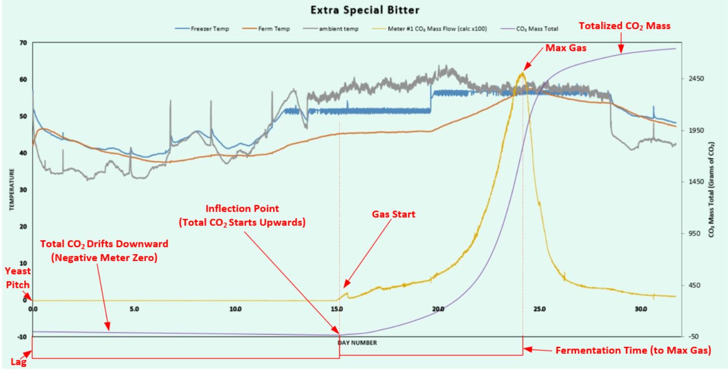 Negative Meter-Zero Example - Purple Line is CO2 Mass Total
With lagers the bubbles may start slow. This lack of clarity makes us choose a rigorous way
to assign the "Gas Start" timing. The batches will all be compared to each other, so these
values must be unambigously determined. For this you need to know if the meter zero was
positive or negative. This is seen as a negative or positive value for the beginning values
in the Meter #1 (cal table) raw data in column H. Once you run through this a couple of
times, you will find that this is not a big deal.
Easiest is negative! If the first Meter #1 values (cell H4 and on) are negative, then the
CO2 Mass Total (probably column Q) is going to build in a negative direction until
the bubbles start. At this point the gas total will start building in a positive direction
until the end. So we are looking for most negative gas mass total value in column Q. After
this, the bubbles will drive the remaining entries higher.
You need to use Excel™ to find the most negative value in column Q, and the day number this
occured on. First, split the screen on the worksheet to find the last row of data. This
row number could be anything depending on how long the batch data capture was run. At the
very bottom of column Q, you want it to look like this:
Min: -0.321752154
Cell with Min: $Q$48
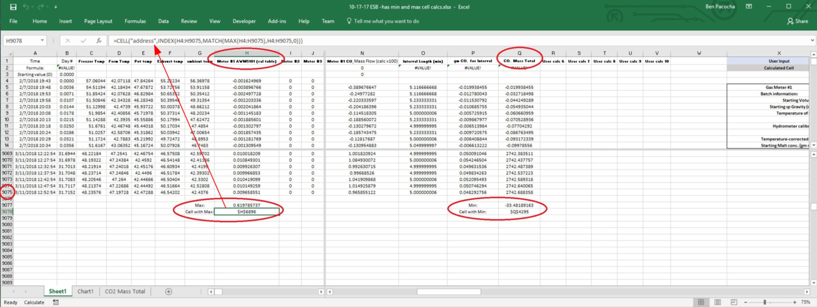 Batch Data With Min and Max Calculations
The Excel™ formula for Min is:
=MIN(Q5:Q1275)
...with Q1275 being replaced with the last cell of data in your sheet. Let's say our new
batch sheet has data until Q9075:
=MIN(Q5:Q9075)
The Excel™ formula for the cell address that contains the Min is:
=CELL("address",INDEX(Q5:Q1275,MATCH(MIN(Q5:Q1275),Q5:Q1275,0)))
...replace any occurrence of 1275 with 9075 (3 spots), and place that formula in the sheet:
=CELL("address",INDEX(Q5:Q9075,MATCH(MIN(Q5:Q9075),Q5:Q9075,0)))
You now know what the minimum was in column Q, and where to find it. Place the Minimum
value in the Batch Score spread sheet. Get to the row specified for the Min, and also
place the Day number for that row in the spread sheet (copy the number from the batch
sheet and paste "values" into the Batch Score sheet.
For a positive meter zero (beginning Meter #1 values (cell H4 and on) are positive):
This is a little harder, because there is no clear inflection point in the gas mass total
from negative to positive values. The mass total increments slowly when there are no
bubbles, then quickens when the fermentation starts. The best we can do in this case is
to use a fraction of the ending mass total to derive the "Gas Start" timing. I am getting
good results using 0.25% of the ending mass total. This places the gas start where you
can see things start to happen on the graph. You can choose a different value, but you
have to use the same value for all of your batches that you are comparing.
The process is:
multiply the ending mass total by 0.0025 (0.25%). This gives you a starting mass total to
search for in Column Q. Find the two rows with values lower and higher then the calculated
one. The row with the lower one is your "Gas Start" row.
In the Amber IPA data, my last row of data is row 6131. The Mass Total value (for Meter #1)
in cell Q6131 is: 3082.690214
3082.690214 x .0025 = 7.71 grams CO2
Looking for the 7.71 value in the rows of column Q, I find that it is reached between rows
348 & 349. So, I will use row 348 as the gas start row for the Batch Score sheet. You can
comfirm this day number value makes sense by looking at the graph.
Max Gas
The maximum gas is the peak gas flow achieved in the raw meter data (Column H for Meter #1).
All you have to do here is run the Excel™ formula to find the max value in column H,
navigate to that row, and document this rate and its corresponding Day Number value in the
Batch Score sheet.
You want the bottom of the data in column H to look like this:
Max: 0.371920074
Cell with Max: $H$3384
Max formula:
=MAX(H4:H6131)
Address of Cell with Max formula:
=CELL("address",INDEX(H4:H6131,MATCH(MAX(H4:H6131),H4:H6131,0)))
In this case, my Max rate is found in cell H3384. Once I navigate to that row, I need to also
record the day number and fermentation temperature into the Batch Score sheet. The ferm
temperature is in column D on the Amber IPA example sheet.
Notes:
For the batches to compare to each other, the run settings have to match. For example, a 1-minute
row interval will give a higher peak flow rate then a 5-minute row interval. These two cannot
be compared in the same Batch Score sheet.
Excel™ Formulas for Max Gas calculation:
Max Gas (maximum individual meter reading; column H for meter 1):
=MAX(H4:H6131)
=CELL("address",INDEX(H4:H6131,MATCH(MAX(H4:H6131),H4:H6131,0)))
Minimum (Min meter mass total for negative meter zero case; column Q in examples):
=MIN(Q5:Q9075)
=CELL("address",INDEX(Q5:Q9075,MATCH(MIN(Q5:Q9075),Q5:Q9075,0)))